The RSM–genetic algorithm gun-drilling study by Han and colleagues optimizes two chip-related responses for a defined copper setup. Reading the complete paper changes the practical question from “what is the best drilling setting?” to “which measured responses did this fitted model improve, within what experimental region?”
The experiment behind the model
The 2025 Materials paper specifies TU1 oxygen-free copper, a 10 mm Botek Type 113 solid-carbide gun drill and a hole length-to-diameter ratio of 50. Coolant enters through the tool and carries chips back along the V-shaped flute. The method identifies a KB1300 machine and ZR-106 emulsified cutting oil.
Its three experimental factors are feed per revolution, cutting speed and cutting-fluid pressure. Table 3 gives these study ranges:
| Factor | Low | Centre | High |
|---|---|---|---|
| Feed, mm/rev | 0.012 | 0.018 | 0.024 |
| Cutting speed, m/min | 47.124 | 54.978 | 62.832 |
| Fluid pressure, MPa | 1.8 | 2.1 | 2.4 |
These are experimental settings for the identified setup, not a copper drilling recommendation. The article describes 27 holes across three specimens, whereas its response-design table contains 17 rows. The allocation of all holes to those rows is not explained in the passages reviewed.
What the responses measure
The paper defines chip volume ratio R in terms of chip occupancy relative to removed metal. CCR uses measured chip thickness relative to the theoretical uncut thickness. Both are constructed chip indicators; neither directly reports bore straightness, tool-life cost or total machine energy.
Table 4 includes five rows at the same central settings with different responses. This makes the observed repeat variation relevant to interpreting a fitted optimum. A higher regression fit alone does not explain that physical variation or remove it from future trials.
RSM fits; the genetic algorithm searches
The response-surface model relates the three selected factors to R and CCR, including interaction terms. The genetic algorithm then searches those fitted relationships inside the specified bounds. It does not directly observe chips or run the machine each time it evaluates a candidate.
The authors prioritize lower R when choosing among candidate trade-offs. That choice belongs to their stated objective. A production problem that also constrains geometric quality or service intervals needs those additional responses represented explicitly.
Prediction and confirmation are separate results
Section 5.1 reports the chosen model solution; section 5.2 describes a nearby feasible setting used for physical confirmation. The reported physical responses differ from the model responses. Preserve both sets rather than presenting predicted values as measured results.
The abstract and conclusion call a value in m/min “spindle speed”; the methods and factor table identify it as cutting speed. Use the unit and the method definition when converting to rpm. The converter below performs that arithmetic, not optimization.
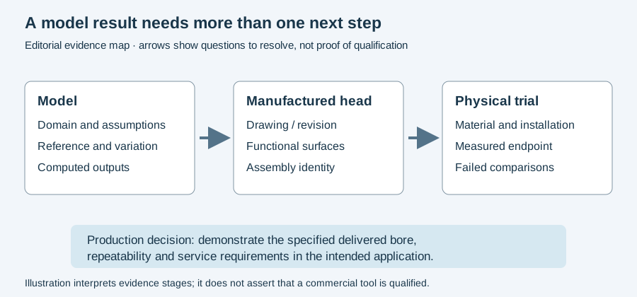
The authors also discuss the risk that model error can direct the algorithm toward a false optimum and that predictions outside the sampled region are unreliable. For a new job, keep the experiment, model, candidate search and physical confirmation as four visible steps. Continue to the methods comparison for experiment design, or feed selection for the quantity and chip interpretation.
Revision note
October 8, 2026: revised the technical explanation and connected reading after source review. Original publication date and URL retained.